Introduction to Generative Adversarial Network

Introduction

Generative Adversarial Networks is an unsupervised model that generates samples indistinguishable samples from the training samples. To generate new samples, the main network, generator generates new sample from a latent variable (a random noise), and a second network known as discriminator is used to discriminate between the real and generated samples. The output of the discriminator is used to train the generator so that the generator can fool the discriminator by generating plausible samples.

Discriminator as a similarity signal

The goal of the GAN is to generate plausible samples ${x_i^f}$, that are indistinguishable from true training data \(\{x_i\}\). A new sample \(x_i^f\) is generated by feeding the latent variable \(z_i\) from a simple base distribution to the generator network, \(g(z_i, \phi)\) with parameters \(\phi\). The learning process involves the optimization of variable \(\phi\) so that generated samples \(\{x_i^f\}\) is similar to \(\{x_i\}\). To quantify the notion of plausibility, GAN uses an additional network a discriminator, \(f(x, \theta)\) to classify whether an image is generated by a generator or from true samples. The discriminator is used to provide a signal that can be used to improve the generation process.

Loss function

The discriminator is trained to optimize a binary classification task, whether the data is from the training set or generated by a generator. The discriminator maximizes the probability of assigning the correct label to both training examples and samples obtained from the generator i.e. maximize \(log(D(x)) + log (1 - D(G(z)))\). However, during implementation, we minimize the traditional binary classification problem:

where, \(y_i \in \{0, 1\}\) is the label. We assume that real examples from the training dataset have label \(y = 1\) and the generated sample have label \(y = 0\), then the above equation can be written as:

In contrast with the discriminator, the generator maximizes the negative log probability of score predicted by the discriminator \(log(1 - f(g(z, \phi), \theta))\) i.e. it seeks to generate a sample that is misclassified by the discriminator. Now, the overall loss function can be formulated as:

\(\phi^*, \theta^* = \underset{\phi}{\operatorname{argmax}} \{ \underset{\theta}{\operatorname{min}} \sum_i- log \text{ } f(x, \theta) - \text{ } log (1 - f(g(z, \phi), \theta)) \}\)

Implementation of GAN

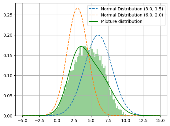
In this section, we implement a simple GAN network in PyTorch. We generate data by sampling from a mixture of Gaussian distribution. We optimize GAN to generate data that mimics the initial distribution of the dataset.

We create two multi-layer perceptron networks for the generator and discriminator and use SGD optimizer to optimize the loss function for each generator and discriminator simultaneously. We define the networks for both the generator and discriminator. The code for training GAN is provided below:

class Generator(nn.Module):
	def __init__(self):
		super().__init__()		
		self.layer_1 = nn.Linear(1, 3, bias=True)
		self.layer_2 = nn.Linear(3, 1, bias = True)

	def forward(self, x):	
		return self.layer_2(F.relu(self.layer_1(x)))

class Discriminator(nn.Module):
	def __init__(self):
		super().__init__()		
		self.weight = nn.Linear(1, 1, bias=True)

	def forward(self, x):
		return F.sigmoid(self.weight(x))

Now, we implement the training loop for the generator and discriminator.

n_epochs = 50
for epoch in range(n_epochs):
    generator_loss = 0
    discriminator_loss = 0
    for data in data_loader:
        data = data.view(-1, 1).to(device)
        batch_size = data.shape[0]

        valid = torch.ones(size=(batch_size, 1), requires_grad=False).to(device)
        fake = torch.zeros(size=(batch_size, 1), requires_grad=False).to(device)

        optimizer_generator.zero_grad()
        z = torch.normal(0, 1, size = (batch_size, 1)).to(device)
        x_f = generator(z)
        prediction_discriminator = discriminator(x_f)
        loss_generator = F.binary_cross_entropy(prediction_discriminator, valid, reduction='mean')
        loss_generator.backward()
        optimizer_generator.step()
        generator_loss += loss_generator.item()

        optimizer_discriminator.zero_grad()
        prediction_generated = discriminator(x_f.detach())
        prediction_true = discriminator(data)
        loss_discriminator = (F.binary_cross_entropy(prediction_generated, fake, reduction='mean') + \
                                F.binary_cross_entropy(prediction_true, valid, reduction='mean')) / 2

        loss_discriminator.backward()
        optimizer_discriminator.step()
        discriminator_loss += loss_discriminator.item()

    print(f"Epoch: {epoch} Loss: ({generator_loss / batch_size}, {discriminator_loss / batch_size})")

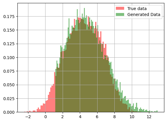
After training the GAN, we visualize the actual distribution and the distribution of samples generated by the generator. As we can see from the figure below that the synthetic data samples generated almost mimics the actual distribution of the dataset.